Radar has landed - discover the latest DDoS attack trends. Get ahead, stay protected.Get the report
Under attack?

Products

Solutions

Resources

Partners

Why Gcore

  1. Home
  2. Developers
  3. What Is a Load Balancer? | How Do Load Balancers Work?

What Is a Load Balancer? | How Do Load Balancers Work?

  • By Gcore
  • June 6, 2023
  • 6 min read
What Is a Load Balancer? | How Do Load Balancers Work?

Have you ever wondered how a web application can scale to serve millions of users worldwide? To serve a vast number of user requests, web applications must build their services to multiple instances. You might then wonder: How can an application evenly distribute the user requests so that all the user requests can be handled with peak efficiency? The short answer to that question is load balancing. The complete answer is…well, please reserve a few minutes to go through the article! You will learn all about load balancing: what a load balancer is, how it works, its benefits, methods of load balancing, and how to implement a load balancer for your use cases.

What Is a Load Balancer?

A load balancer is a hardware device or software application responsible for evenly distributing the requests across multiple application instances. (An “instance” is a single deployment of an application or service running on a server.) As a result, the application can cope with a high volume of requests efficiently.

If an additional app instance is introduced, the load balancer will redistribute the requests to include the new instance, thus reducing the workload on the existing instances. If an app instance goes down, all the requests to the problematic instance will be redistributed to other operational instances. As a result, the app is highly available and fault tolerant, offering users an uninterrupted service.

Load balancers can be categorized into different types based on how they manage and redistribute incoming requests. The two primary types are network load balancers, and application load balancers. Another mode of categorization is by physicality type, in which case we divide them into hardware and software load balancers. Let’s take a look at each of these in depth.

Network Load Balancers

Network load balancers forward the requests at the transport layer, layer 4 of the Open System Interconnection (OSI) model. The forwarding mechanism is based solely on network attributes, such as the IP addresses of the clients and the corresponding application instances.

Network balancers do not consider the contents of the requests when forwarding them to the app instances, which allows them to offer low latencies when redistributing the requests. Network load balancers would be a great fit for applications with extreme performance requirements, such as streaming or game applications.

Application Load Balancers

Application load balancers forward the requests at the application layer, also known as layer 7 of the OSI model. They examine the content of the requests, such as HTTP Headers, request paths, or request methods. This way, the application load balancer can flexibly distribute the requests to different app instances to match the business requirements.

Application load balancers are appropriate for e-commerce or social network applications that need support for custom HTTP responses and health checks for the app instances but do not require extremely low latencies.

Hardware Load Balancers

Network and application are categories of load balancers based on how they manage and redistribute incoming requests.

Hardware load balancers are purpose-built devices designed to redistribute the requests among app instances. They are often used in on-premise infrastructure alongside the company’s network systems and application servers. Hardware load balancers are a good choice for applications that want to store all data in self-managed servers or require special hardware customization when forwarding the requests to the target instances. They also offer enhanced security options.

Benefits of a Load Balancer

A load balancer can help with application performance in a number of ways, including scalability, cost reduction, availability, and request processing speed. Let’s take a closer look at each of these in turn.

Scalability

When more user requests are sent to the application server instances, the CPU utilization of the server instances is high.

An e-commerce application would benefit from the scalability the load balancers offer. Typically, the volume of user requests for e-commerce applications escalates far above normal levels during Black Friday sales.

High Availability

If one application instance goes down, the load balancer will forward the requests to other instances so the end user does not encounter any error or stoppage in service. The load balancer helps to ensure an application’s high availability by circumventing problematic instances.

How Load Balancing Works

To create a load balancing system that effectively forwards requests to the application instances, it’s first essential to understand how a load balancer works. Let’s review the inner workings of load balancing and explore some popular load balancing methods.

How Does a Load Balancer Work?

Different algorithms and combinations thereof are used by load balancers. The algorithm(s) depend on the complexity and features of the load balancer in question. A basic load balancer usually uses an algorithm called Round Robin to assign requests to the app instances. The Round Robin algorithm distributes the requests to the app instances one-by-one, resulting in an equal load distribution. No single app is overly taxed.

Let’s say you have three application instances. The first user request will be sent to instance number one. The second request will be sent to instance number two. The third request will be sent to instance number three. The fourth request will be sent to instance number four. Here, we have four instances available, so request number five will be sent to app instance one, and so on.

Figure 1: Demonstration of how a load balancer works

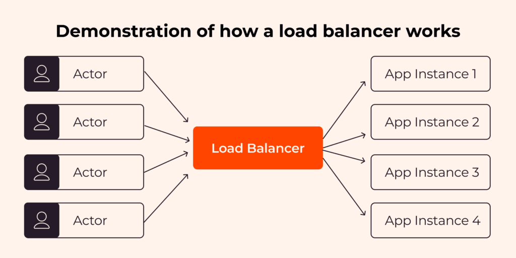
Instead of interacting directly with the application server, your application’s end users send requests to the load balancer.

What Are the Components of a Load Balancer?

A typical load balancer consists of four parts:

  1. Virtual IP: This is the unique digital address of the load balancer, allowing the client to send requests to the load balancer.
  2. Network protocols: Different types of load balancers support different network protocols. For example, a network load balancer supports TCP or UDP protocol, whereas an application load balancer supports HTTP and HTTPS protocols.
  3. Load balancing algorithms: Load balancers use different algorithms, such as Round Robin and IP Hash, to determine to which appropriate application instance they should forward the client’s request.
  4. Health monitoring: The load balancer routinely checks the health status of each app instance.

Load Balancing Methods

Besides the Round Robin algorithm already discussed, other load balancing methods and algorithms exist, including Weighted Round Robin and resourced-based methods. In general, the load-balancing methods can be divided into two categories: static load balancing and dynamic load balancing. Let’s take a closer look at each.

Static Load Balancing

With static load balancing, the load balancers forward the requests to the app instances without examining the current state of these app instances. This makes static load balancing easy to implement. The drawback of the static load balancing method is that it cannot adapt to the states of the app instances, which could be very different in runtime from what you anticipated, potentially affecting performance, and thus user experience. Some static load balancing methods are:

  • Round Robin: The load balancer will forward the requests to the app instances cyclically, distributing requests evenly across the instances.
  • Weighted Round Robin: Each app instance is assigned a weight, serving as an indicator of its processing capacity or priority. The load balancer forwards requests to the app instances according to the weighting. The higher the weighted number the app instance has, the more requests will be forwarded to that instance.
  • IP hash: The load balancer generates a unique hash key based on both the client IP and the app instance IP. This method allows the client to interact with the same app instance repeatedly across multiple sessions. IP hash load balancing algorithm is suitable for applications that need persisted sessions between the client and the app instance because they ensure a continuous, seamless experience for the user.

Dynamic Load Balancing

With dynamic load balancing, load balancers forward requests to the app instances based on the current state of these instances. As a result, the dynamic load balancers can adapt to the ongoing changes of the app instances and tend to be more efficient than the static load balancers. However, dynamic load balancing is more complicated to implement. Some examples of dynamic load balancing methods are:

  • Least connection: With the least connection load balancing method, the requests are forwarded to the app instance with the lowest number of active connections.
  • Weighted least connection: The weighted least connection method will forward the requests to the app instance based on the number of active connections and the weighting of that instance. For example, if there are three app instances with the same number of active connections, the one with the highest weighting number will be chosen to forward the request.

Load Balancer in the Cloud

Setting up and maintaining a group of load balancers is a challenging task. To create and manage load balancers efficiently, you need to:

  • Have a number of different load-balancing algorithms to support different internal business use cases
  • Monitor your system health for the application instances
  • Configure access controls and protection for your load balancers to prevent malicious access from the public internet
  • Ensure scalability of your load balancer as your application needs grow

Gcore’s Load Balancer

At Gcore, we understand the difficulties and challenges of setting up a load balancer from scratch. There are a huge number of options available, and your choice directly affects performance and user experience—for better or for worse. Gcore’s Load Balancer solves these challenges and comes with built-in features support for:

  • Different load balancing algorithms such as Round Robin, least connections, and source IP, so that you can choose the one that fits your need
  • Setting up unhealthy and healthy thresholds
  • Setting up the load balancers firewall, which allows you to set the rules for inbound and outbound traffic to enhance security

To learn more about how to get started, configure, and troubleshoot the Gcore Load Balancer, please take a look at our knowledge page.

Conclusion

With a growing number of users coming to your app, having a load balancer to distribute user requests to your instances appropriately is essential for performance and user experience. However, setting up a load balancer that appropriately distributes user requests takes a lot of work. The Gcore Load Balancer helps you to distribute your user workload in the most elegant and efficient way possible.

Related articles

How to get the size of a directory in Linux

Understanding how to check directory size in Linux is critical for managing storage space efficiently. Understanding this process is essential whether you’re assessing specific folder space or preventing storage issues.This comprehensive guide covers commands and tools so you can easily calculate and analyze directory sizes in a Linux environment. We will guide you step-by-step through three methods: du, ncdu, and ls -la. They’re all effective and each offers different benefits.What is a Linux directory?A Linux directory is a special type of file that functions as a container for storing files and subdirectories. It plays a key role in organizing the Linux file system by creating a hierarchical structure. This arrangement simplifies file management, making it easier to locate, access, and organize related files. Directories are fundamental components that help ensure smooth system operations by maintaining order and facilitating seamless file access in Linux environments.#1 Get Linux directory size using the du commandUsing the du command, you can easily determine a directory’s size by displaying the disk space used by files and directories. The output can be customized to be presented in human-readable formats like kilobytes (KB), megabytes (MB), or gigabytes (GB).Check the size of a specific directory in LinuxTo get the size of a specific directory, open your terminal and type the following command:du -sh /path/to/directoryIn this command, replace /path/to/directory with the actual path of the directory you want to assess. The -s flag stands for “summary” and will only display the total size of the specified directory. The -h flag makes the output human-readable, showing sizes in a more understandable format.Example: Here, we used the path /home/ubuntu/, where ubuntu is the name of our username directory. We used the du command to retrieve an output of 32K for this directory, indicating a size of 32 KB.Check the size of all directories in LinuxTo get the size of all files and directories within the current directory, use the following command:sudo du -h /path/to/directoryExample: In this instance, we again used the path /home/ubuntu/, with ubuntu representing our username directory. Using the command du -h, we obtained an output listing all files and directories within that particular path.#2 Get Linux directory size using ncduIf you’re looking for a more interactive and feature-rich approach to exploring directory sizes, consider using the ncdu (NCurses Disk Usage) tool. ncdu provides a visual representation of disk usage and allows you to navigate through directories, view size details, and identify large files with ease.For Debian or Ubuntu, use this command:sudo apt-get install ncduOnce installed, run ncdu followed by the path to the directory you want to analyze:ncdu /path/to/directoryThis will launch the ncdu interface, which shows a breakdown of file and subdirectory sizes. Use the arrow keys to navigate and explore various folders, and press q to exit the tool.Example: Here’s a sample output of using the ncdu command to analyze the home directory. Simply enter the ncdu command and press Enter. The displayed output will look something like this:#3 Get Linux directory size using 1s -1aYou can alternatively opt to use the ls command to list the files and directories within a directory. The options -l and -a modify the default behavior of ls as follows:-l (long listing format)Displays the detailed information for each file and directoryShows file permissions, the number of links, owner, group, file size, the timestamp of the last modification, and the file/directory name-a (all files)Instructs ls to include all files, including hidden files and directoriesIncludes hidden files on Linux that typically have names beginning with a . (dot)ls -la lists all files (including hidden ones) in long format, providing detailed information such as permissions, owner, group, size, and last modification time. This command is especially useful when you want to inspect file attributes or see hidden files and directories.Example: When you enter ls -la command and press Enter, you will see an output similar to this:Each line includes:File type and permissions (e.g., drwxr-xr-x):The first character indicates the file type- for a regular filed for a directoryl for a symbolic linkThe next nine characters are permissions in groups of three (rwx):r = readw = writex = executePermissions are shown for three classes of users: owner, group, and others.Number of links (e.g., 2):For regular files, this usually indicates the number of hard linksFor directories, it often reflects subdirectory links (e.g., the . and .. entries)Owner and group (e.g., user group)File size (e.g., 4096 or 1045 bytes)Modification date and time (e.g., Jan 7 09:34)File name (e.g., .bashrc, notes.txt, Documents):Files or directories that begin with a dot (.) are hidden (e.g., .bashrc)ConclusionThat’s it! You can now determine the size of a directory in Linux. Measuring directory sizes is a crucial skill for efficient storage management. Whether you choose the straightforward du command, use the visual advantages of the ncdu tool, or opt for the versatility of ls -la, this expertise enhances your ability to uphold an organized and efficient Linux environment.Looking to deploy Linux in the cloud? With Gcore Edge Cloud, you can choose from a wide range of pre-configured virtual machines suitable for Linux:Affordable shared compute resources starting from €3.2 per monthDeploy across 50+ cloud regions with dedicated servers for low-latency applicationsSecure apps and data with DDoS protection, WAF, and encryption at no additional costGet started today

How to Run Hugging Face Spaces on Gcore Inference at the Edge

Running machine learning models, especially large-scale models like GPT 3 or BERT, requires a lot of computing power and comes with a lot of latency. This makes real-time applications resource-intensive and challenging to deliver. Running ML models at the edge is a lightweight approach offering significant advantages for latency, privacy, and resource optimization.  Gcore Inference at the Edge makes it simple to deploy and manage custom models efficiently, giving you the ability to deploy and scale your favorite Hugging Face models globally in just a few clicks. In this guide, we’ll walk you through how easy it is to harness the power of Gcore’s edge AI infrastructure to deploy a Hugging Face Space model. Whether you’re developing NLP solutions or cutting-edge computer vision applications, deploying at the edge has never been simpler—or more powerful. Step 1: Log In to the Gcore Customer PortalGo to gcore.com and log in to the Gcore Customer Portal. If you don’t yet have an account, go ahead and create one—it’s free. Step 2: Go to Inference at the EdgeIn the Gcore Customer Portal, click Inference at the Edge from the left navigation menu. Then click Deploy custom model. Step 3: Choose a Hugging Face ModelOpen huggingface.com and browse the available models. Select the model you want to deploy. Navigate to the corresponding Hugging Face Space for the model. Click on Files in the Space and locate the Docker option. Copy the Docker image link and startup command from Hugging Face Space. Step 4: Deploy the Model on GcoreReturn to the Gcore Customer Portal deployment page and enter the following details: Model image URL: registry.hf.space/ethux-mistral-pixtral-demo:latest Startup command: python app.py Container port: 7860 Configure the pod as follows: GPU-optimized: 1x L40S vCPUs: 16 RAM: 232GiB For optimal performance, choose any available region for routing placement. Name your deployment and click Deploy.Step 5: Interact with Your ModelOnce the model is up and running, you’ll be provided with an endpoint. You can now interact with the model via this endpoint to test and use your deployed model at the edge.Powerful, Simple AI Deployment with GcoreGcore Inference at the Edge is the future of AI deployment, combining the ease of Hugging Face integration with the robust infrastructure needed for real-time, scalable, and global solutions. By leveraging edge computing, you can optimize model performance and simultaneously futureproof your business in a world that increasingly demands fast, secure, and localized AI applications. Deploying models to the edge allows you to capitalize on real-time insights, improve customer experiences, and outpace your competitors. Whether you’re leading a team of developers or spearheading a new AI initiative, Gcore Inference at the Edge offers the tools you need to innovate at the speed of tomorrow. Explore Gcore Inference at the Edge

10 Common Web Performance Mistakes and How to Overcome Them

Web performance mistakes can carry a high price, resulting in websites that yield low conversion rates, high bounce rates, and poor sales. In this article, we dig into the top 10 mistakes you should avoid to boost your website performance.1. Slow or Unreliable Web HostYour site speed begins with your web host, which provides the server infrastructure and resources for your website. This includes the VMs and other infrastructure where your code and media files reside. Three common host-related problems are as follows:Server location: The further away your server is from your users, the slower the site speed and the poorer the experience for your website visitors. (More on this under point 7.)Shared hosting: Shared hosting solutions share server resources among multiple websites, leading to slow load times and spotty connections during peak times due to heavy usage. Shared VMs can also impact your website’s performance due to increased network traffic and resource contention.VPS hosting: Bandwidth limitations can be a significant issue with VPS hosting. A limited bandwidth package can cause your site speed to decrease during high-traffic periods, resulting in a sluggish user experience.Correct for server and VM hosting issues by choosing a provider with servers located closer to your user base and provisioning sufficient computational resources, like Gcore CDN. Use virtual dedicated servers (VDS/VPS) rather than shared hosting to avoid network traffic from other websites affecting your site’s performance. If you already use a VPS, consider upgrading your hosting plan to increase server resources and improve UX. For enterprises, dedicated servers may be more suitable.2. Inefficient Code, Libraries, and FrameworksPoor-quality code and inefficient frameworks can increase the size of web pages, consume too many resources, and slow down page load times. Code quality is often affected by syntax, semantics, and logic errors. Correct these issues by writing clean and simple code.Errors or inefficiencies introduced by developers can impact site performance, such as excessive API calls or memory overuse. Prevent these issues by using TypeScript, console.log, or built-in browser debuggers during development. For bugs in already shipped code, utilize logging and debugging tools like the GNU debugger or WinDbg to identify and resolve problems.Improving code quality also involves minimizing the use of large libraries and frameworks. While frontend frameworks like React, Vue, and Angular.js are popular for accelerating development, they often include extensive JavaScript and prebuilt components that can bloat your website’s codebase. To optimize for speed, carefully analyze your use case to determine if a framework is necessary. If a static page suffices, avoid using a framework altogether. If a framework is needed, select libraries that allow you to link only the required components.3. Unoptimized Code Files and FontsEven high-quality code needs optimization before shipping. Unoptimized JavaScript, HTML, and CSS files can increase page weight and necessitate multiple HTTP requests, especially if JavaScript files are executed individually.To optimize code, two effective techniques are minification and bundling.Minification removes redundant libraries, code, comments, unnecessary characters (e.g., commas and dots), and formatting to reduce your source code’s size. It also shortens variable and function names, further decreasing file size. Tools for minification include UglifyJS for JavaScript, CSSNano for CSS, and HTMLminifier for HTML.Bundling groups multiple files into one, reducing the number of HTTP requests and speeding up site load times. Popular bundling tools include Rollup, Webpack, and Parcel.File compression using GZIP or Brotli can also reduce the weight of HTTP requests and responses before they reach users’ browsers. Enable your chosen compression technique on your server only after checking that your server provider supports it.4. Unoptimized Images and VideosSome websites are slowed down by large media files. Upload only essential media files to your site. For images, compress or resize them using tools like TinyPNG and Compressor.io. Convert images from JPEG, PNG, and GIF to WebP and AVIF formats to maintain quality while reducing file size. This is especially beneficial in industries like e-commerce and travel, where multiple images boost conversion rates. Use dynamic image optimization services like Gcore Image Stack for efficient processing and delivery. For pages with multiple images, use CSS sprites to group them, reducing the number of HTTP requests and speeding up load times.When adding video files, use lite embeds for external links. Standard embed code, like YouTube’s, is heavy and can slow down your pages. Lite embeds load only thumbnail images initially, and the full video loads when users click the thumbnail, improving page speed.5. No Lazy LoadingLazy loading delays the rendering of heavy content like images and JavaScript files until the user needs it, contrasting with “eager” loading, which loads everything at once and slows down site load times. Even with optimized images and code, lazy loading can further enhance site speed through a process called “timing.”Image timing uses the HTML loading attribute in an image tag or frameworks like Angular or React to load images in response to user actions. The browser only requests images when the user interacts with specific features, triggering the download.JavaScript timing controls when certain code loads. If JavaScript doesn’t need to run until the entire page has rendered, use the defer attribute to delay its execution. If JavaScript can load at any time without affecting functionality, load it asynchronously with the async attribute.6. Heavy or Redundant External Widgets and PluginsWidgets and plugins are placed in designated frontend and backend locations to extend website functionality. Examples include Google review widgets that publish product reviews on your website and Facebook plugins that connect your website to your Facebook Page. As your website evolves, more plugins are typically installed, and sometimes website admins forget to remove those that are no longer required.Over time, heavy and unused plugins can consume substantial resources, slowing down your website unnecessarily. Widgets may also contain heavy HTML, CSS, or JavaScript files that hinder web performance.Remove unnecessary plugins and widgets, particularly those that make cURL calls, HTTP requests, or generate excessive database queries. Avoid plugins that load heavy scripts and styles or come from unreliable sources, as they may contain malicious code and degrade website performance.7. Network IssuesYour server’s physical location significantly impacts site speed for end users. For example, if your server is in the UK and your users are in China, they’ll experience high latency due to the distance and DNS resolution time. The greater the distance between the server and the user, the more network hops are required, increasing latency and slowing down site load times.DNS resolution plays a crucial role in this process. Your authoritative DNS provider resolves your domain name to your IP address. If the provider’s server is too far from the user, DNS resolution will be slow, giving visitors a poor first impression.To optimize content delivery and reduce latency, consider integrating a content delivery network (CDN) with your server-side code. A CDN stores copies of your static assets (e.g., container images, JavaScript, CSS, and HTML files) on geographically distributed servers. This distribution ensures that users can access your content from a server closer to their location, significantly improving site speed and performance.8. No CachingWithout caching, your website has to fetch data from the origin server every time a user requests. This increases the load time because the origin server is another physical hop that data has to travel.Caching helps solve this problem by serving pre-saved copies of your website. Copies of your web files are stored on distributed CDN servers, meaning they’re available physically closer to website viewers, resulting in quicker load times.An additional type of caching, DNS caching, temporarily stores DNS records in DNS resolvers. This allows for faster domain name resolution and accelerates the initial connection to a website.9. Excessive RedirectsWebsite redirects send users from one URL to another, often resulting in increased HTTP requests to servers. These additional requests can potentially crash servers or cause resource consumption issues. To prevent this, use tools like Screaming Frog to scan your website for redirects and reduce them to only those that are absolutely necessary. Additionally, limit each redirect to making no more than one request for a .css file and one for a .js file.10. Lack of Mobile OptimizationForgetting to optimize for mobile can harm your website’s performance. Mobile-first websites optimize for speed and UX. Better UX leads to happier customers and increased sales.Optimizing for mobile starts with understanding the CPU, bandwidth, and memory limitations of mobile devices compared to desktops. Sites with excessively heavy files will load slowly on mobiles. Writing mobile-first code, using mobile devices or emulators for building and testing, and enhancing UX for various mobile device types—such as those with larger screens or higher capacity—can go a long way to optimizing for mobile.How Can Gcore Help Prevent These Web Performance Mistakes?If you’re unsure where to start in correcting or preventing web performance mistakes, don’t worry—you don’t have to do it alone. Gcore offers a comprehensive suite of solutions designed to enhance your web performance and deliver the best user experience for your visitors:Powerful VMs: Fast web hosting with a wide range of virtual machines.Managed DNS: Hosting your DNS zones and ensuring quick DNS resolution with our fast Managed DNS.CDN: Accelerate both static and dynamic components of your website for global audiences.With robust infrastructure from Gcore, you can ensure optimal performance and a seamless experience for all your web visitors. Keep your website infrastructure in one place for a simplified website management experience.Need help getting started? Contact us for a personalized consultation and discover how Gcore can supercharge your website performance.Get in touch to boost your website

How to Choose Between Bare Metal GPUs and Virtual GPUs for AI Workloads

Choosing the right GPU type for your AI project can make a huge difference in cost and business outcomes. The first consideration is often whether you need a bare metal or virtual GPU. With a bare metal GPU, you get a physical server with an entire GPU chip (or chips) installed that is completely dedicated to the workloads you run on the server, whereas a virtual GPU means you share GPU resources with other virtual machines.Read on to discover the key differences between bare metal GPUs and virtual GPUs, including performance and scalability, to help you make an informed decision.The Difference Between Bare Metal and Virtual GPUsThe main difference between bare metal GPUs and virtual GPUs is how they use physical GPU resources. With a bare metal GPU, you get a physical server with an entire GPU chip (or chips) installed that is completely dedicated to the workloads you run on the server. There is no hypervisor layer between the operating system (OS) and the hardware, so applications use the GPU resources directly.With a virtual GPU, you get a virtual machine (VM) and uses one of two types of GPU virtualization, depending on your or a cloud provider’s capabilities:An entire, dedicated GPU used by a VM, also known as a passthrough GPUA shared GPU used by multiple VMs, also known as a vGPUAlthough a passthrough GPU VM gets the entire GPU, applications access it through the layers of a guest OS and hypervisor. Also, unlike a bare metal GPU instance, other critical VM resources that applications use, such as RAM, storage, and networking, are also virtualized.The difference between running applications with bare metal and virtual GPUsThese architectural features affect the following key aspects:Performance and latency: Applications running on a VM with a virtual GPU, especially vGPU, will have lower processing power and higher latency for the same GPU characteristics than those running on bare metal with a physical GPU.Cost: As a result of the above, bare metal GPUs are more expensive than virtual GPUs.Scalability: Virtual GPUs are easier to scale than bare metal GPUs because scaling the latter requires a new physical server. In contrast, a new GPU instance can be provisioned in the cloud in minutes or even seconds.Control over GPU hardware: This can be critical for certain configurations and optimizations. For example, when training massive deep learning models with a billion parameters, total control means the ability to optimize performance optimization—and that can have a big impact on training efficiency for massive datasets.Resource utilization: GPU virtualization can lead to underutilization if the tasks being performed don’t need the full power of the GPU, resulting in wasted resources.Below is a table summarizing the benefits and drawbacks of each approach: Bare metal GPUVirtual GPUPassthrough GPUvGPUBenefitsDedicated GPU resourcesHigh performance for demanding AI workloadsLower costSimple scalabilitySuitable for occasional or variable workloadsLowest costSimple scalabilitySuitable for occasional or variable workloadsDrawbacksHigh cost compared to virtual GPUsLess flexible and scalable than virtual GPUsLow performanceNot suitable for demanding AI workloadsLowest performanceNot suitable for demanding AI workloadsShould You Use Bare Metal or Virtual GPUs?Bare metal GPUs and virtual GPUs are typically used for different types of workloads. Your choice will depend on what AI tasks you’re looking to perform.Bare metal GPUs are better suited for compute-intensive AI workloads that require maximum performance and speed, such as training large language models. They are also a good choice for workloads that must run 24/7 without interruption, such as some production AI inference services. Finally, bare metal GPUs are preferred for real-time AI tasks, such as robotic surgery or high-frequency trading analytics.Virtual GPUs are a more suitable choice for the early stages of AI/ML and iteration on AI models, where flexibility and cost-effectiveness are more important than top performance. Workloads with variable or unpredictable resource requirements can also run on this type of GPU, such as training and fine-tuning small models or AI inference tasks that are not sensitive to latency and performance. Virtual GPUs are also great for occasional, short-term, and collaborative AI/ML projects that don’t require dedicated hardware—for example, an academic collaboration that includes multiple institutions.To choose the right type of GPU, consider these three factors:Performance requirements. Is the raw GPU speed critical for your AI workloads? If so, bare metal GPUs are a superior choice.Scalability and flexibility. Do you need GPUs that can easily scale up and down to handle dynamic workloads? If yes, opt for virtual GPUs.Budget. Depending on the cloud provider, bare metal GPU servers can be more expensive than virtual GPU instances. Virtual GPUs typically offer more flexible pricing, which may be appropriate for occasional or variable workloads.Your final choice between bare metal GPUs and virtual GPUs depends on the specific requirements of the AI/ML project, including performance needs, scalability requirements, workload types, and budget constraints. Evaluating these factors can help determine the most appropriate GPU option.Choose Gcore for Best-in-Class AI GPUsGcore offers bare metal servers with NVIDIA H100, A100, and L40S GPUs. Using the 3.2 Tbps InfiniBand interface, you can combine H100 or A100 servers into scalable GPU clusters for training and tuning massive ML models or for high-performance computing (HPC).If you are looking for a scalable and low-latency solution for global AI inference, explore Gcore Inference at the Edge. It especially benefits latency-sensitive, real-time applications, such as generative AI and object recognition.Discover Gcore bare metal GPUs

How to Configure Grafana for Visualizing Kubernetes (K8s) Cluster Monitoring

Kubernetes monitoring allows you to observe your workloads and cluster resources, spot issues and failures, and efficiently manage pods and other resources. Cluster admins should prioritize tracking the performance and stability of clusters in these environments. One popular tool that can help you visualize Kubernetes monitoring is Grafana. This monitoring solution lets you display K8s metrics through interactive dashboards and real-time alerts. It seamlessly integrates with Prometheus and other data sources, providing valuable insights.Gcore Managed Kubernetes simplifies the Grafana setup process by providing a managed service that includes tools like Grafana. In this article, we’ll explain how to set up and configure Grafana to monitor Kubernetes, its key metrics, and dashboards.Setting Up Grafana for Effective Kubernetes MonitoringTo begin monitoring Kubernetes with Grafana, first, check that you have all the requirements in place: a functioning Kubernetes cluster, the Helm package manager installed, and kubectl set up to communicate with your cluster.Install Grafana in a Kubernetes Cluster. Start by adding the Grafana Helm repository.helm repo add grafana https://grafana.github.io/helm-chartshelm repo updateNext, install Grafana using Helm. This command deploys Grafana into your Kubernetes cluster:helm install grafana grafana/grafanaNow it’s time to configure Grafana for the Kubernetes environment. After installation, retrieve the admin password by using the command below:kubectl get secret --namespace default grafana -o jsonpath="{.data.admin-password}" | base64 --decode ; echoThen access the Grafana UI by port-forwarding:kubectl port-forward svc/grafana 3000:80Open your web browser and navigate to http://localhost:3000. Log in using the default username admin and the password you retrieved. Once logged in, you can configure Grafana to monitor your Kubernetes environment by adding data sources such as Prometheus and creating custom dashboards.You’ve now successfully set up Grafana for Kubernetes monitoring!Key Metrics for Kubernetes MonitoringUnderstanding metrics for Kubernetes monitoring allows you to visualize your cluster’s reliability. Key metrics are the following:Node resources. Track CPU and memory usage, disk utilization, and network bandwidth to understand resource consumption and identify bottlenecks.Cluster metrics. Monitor the number of nodes to understand resource billing and overall cluster usage, and track running pods to determine node capacity and identify failures.Pod metrics. Measure how pods are managed and deployed, including instances and deployment status, and monitor container metrics like CPU, memory, and network usage.State metrics. Keep an eye on persistent volumes, disk pressure, crash loops, and job success rates to ensure proper resource management and application stability.Container metrics. Track container CPU and memory usage relative to pod limits, and monitor network data to detect bandwidth issues.Application metrics. Measure application availability, performance, and business-specific metrics to maintain optimal user experience and operational health.Setting Up Grafana DashboardsYou can opt to design and tailor Grafana dashboards to monitor your Kubernetes cluster. This will help you better understand your systems’ performance and overall well-being at a glance.Log into Grafana. Open your web browser, go to http://localhost:3000/, and log in with the default credentials (admin for both username and password), then change your password if/when prompted.Grafana—Log In to Start MonitoringAdd data source. Navigate to Configuration and select Data Sources. Click on Add Data Source and choose the appropriate data source, such as Prometheus.Create a dashboard. Go to Create > Dashboard, click Add New Panel, choose the panel type (e.g., Time series chart, Gauge, Table), and configure it with a PromQL query and visualization settings.Adding a New Panel in Grafana DashboardOrganize and save the dashboard. Arrange panels by clicking Add Panel > Add Row and dragging panels into the desired rows. To save the dashboard, click the save icon, name it, and confirm the save.Gcore Managed Kubernetes for Kubernetes MonitoringWhether you’re getting started with monitoring Kubernetes or you’re a seasoned pro, Gcore Managed Kubernetes offers significant advantages for businesses seeking efficient and reliable Kubernetes cluster monitoring and container management:Ease of integrating Grafana: The service seamlessly integrates with Grafana, enabling effortless visualization and monitoring of performance metrics via dashboards.Automated control: Gcore Managed Kubernetes simplifies the setup and monitoring process by using automation. This service conducts health checks on your nodes, automatically updating and restarting them when needed to keep performance at its best.Enhanced security and reliability: Gcore Managed Kubernetes guarantees the management of nodes by integrating features like automatic scaling and self-repairing systems to maintain optimal performance.Discover Gcore Managed Kubernetes, including automated scaling, one-click provisioning, and Grafana integration.

TCO Comparison: Self-Managed Kubernetes vs. Managed Kubernetes Provider

Calculating the total cost of ownership (TCO) for Kubernetes requires identifying all major expenses, including infrastructure costs, personnel costs, and potential cloud provider fees. With a clear picture of TCO, you can make a more informed decision when choosing between self-managed (self-hosted) Kubernetes and a managed Kubernetes provider. The TCOs of the two approaches are significantly different, and this article will show you exactly how and why.TCO Comparison SummaryThe table below shows the key aspects of the TCO comparison between self-managed Kubernetes and managed Kubernetes providers. It compares infrastructure expenses, including provider fees, and an engineer’s salary.For this comparison, we’ll assume that a company would need only one DevOps engineer for managed Kubernetes, whereas companies opting for self-hosted Kubernetes would need three. We’ll look at rented cloud VMs for self-hosted, and out-of-the-box K8s clusters for managed Kubernetes—two standard scenarios for a fair comparison. For both scenarios, the infrastructure costs shown in the table are the average when considering AWS, Azure, Google Cloud, and Gcore. InfrastructureEngineers’ salaryTotal annual costSelf-hosted Kubernetes$13,737.64$321,500$335,238Managed Kubernetes$6,157.8$107,167$113,325As you can see, the TCO of self-hosted Kubernetes is almost three times higher than that of managed Kubernetes. Let’s explore the reasons for this major cost discrepancy.Infrastructure Cost ComparisonKubernetes is a free software. But to run it, you have to rent or buy infrastructure, such as VMs or physical servers. The way you do so differs depending on whether you opt for self-hosted or managed Kubernetes. To understand infrastructure costs, we need to take a closer look at each method in turn and explore the components required.Self-hosted KubernetesIf you choose to run K8s independently, you’ll need to rent VMs for the Kubernetes master node (the control plane) and worker nodes. Let’s consider a production-grade cluster consisting of the following:3 VMs for the control plane, required for fault tolerance2 VMs for the worker nodesFor simplicity, we choose VMs with a configuration suitable for an average web project: 8 vCPU, 16 GB RAM, and 75 GB SSD.Here is the pricing* offered by four cloud providers for VMs available in the US:ProviderVM types and resourcesTotal annual cost of five VMsAWSc6g.2xlarge—8 vCPU, 16 GB RAM, 75 GB SSD$12,273.6AzureA8 v2 series—8 vCPU, 16 GB RAM, 64 GB SSD**$17,764.2Google CloudN1 series—8 vCPU, 16 GB RAM, 75 GB SSD$16,721.33Gcoreg1 standard series—8 vCPU, 16 GB RAM, 75 GB SSD$8,191.42Average$13,737.64* Prices are for on-demand VMs; no commitment; no VAT; ingress traffic is not included.** Azure only offers fixed volume sizes for built-in storage.Managed KubernetesWith managed K8s, you don’t have to worry about renting separate VMs and setting up the Kubernetes software. You choose the VM configurations for your worker nodes, and a provider prepares them for you. The result is an out-of-the-box Kubernetes cluster.Sometimes, you also have to consider fees for control plane management (fixed) and egress traffic (consumption-based). Providers like AWS, Google Cloud, and Azure charge for this, while others—like Gcore—don’t.Here are the prices* offered by four cloud providers for similar cluster configurations in the US:ProviderControl plane managementCluster of two worker nodesTotal annual costConfigurationAnnual costAmazon EKS$8768 vCPU, 16 GB RAM, 75 GB SSD$4,909.44$5,785.44AKS (Azure)$8768 vCPU, 16 GB RAM, 64 GB SSD**$7,048.08$7,924.08GKE (Google)$876X vCPUs, X GB RAM$6,832.08$7,708.08Gcore Managed Kubernetes08 vCPU, 16 GB RAM, 75 GB SSD$3,213.6$3,213.6Average$6,157.8* Prices are for on-demand VMs; no commitment; no VAT; ingress traffic is not included.** Azure only offers fixed volume sizes for built-in storage.Engineer Cost ComparisonTo maintain a production-grade cluster for an average web project, you need:For a self-hosted K8s cluster—3 DevOps engineersFor a managed K8s cluster—1 DevOps engineerTo learn more about the technical reasons behind these calculations, read our article on the difference between managed and self-managed Kubernetes.According to Glassdoor, the median salary for a DevOps engineer is as follows:In the US: $140,000In Germany: €69,000 (or $74,333, the highest in Europe) DevOps salary in the USDevOps salary in GermanyAverage annual salarySelf-hosted Kubernetes (3 engineers)$420,000$222,999$321,500Managed Kubernetes (1 engineer)$140,000$74,333$107,167Final ComparisonHere is the final TCO comparison between self-managed Kubernetes and managed Kubernetes providers:ProvidersInfrastructureEngineers’ salaryTotal annual costBy providerAverageSelf-hosted KubernetesAWS$12,273.6$13,737.64$321,500$335,238Azure$17,764.2GCP$16,721.33Gcore$8,191.42Managed KubernetesAmazon EKS$5,785.44$6,157.8$107,167$113,325AKS (Azure)$7,924.08GKE (Google)$7,708.08Gcore Managed Kubernetes$3,213,6Summing UpPlease note that these approximate calculation probably aren’t exactly what you’ll experience. The actual numbers will depend on many factors, including:Size and complexity of your projectLocation where you hire engineers and deploy a K8s clusterChoice of providerHow you consume and scale computing resourcesHowever, the difference between the TCO of the two methods is relevant to what we got above: the total cost of ownership of self-managed Kubernetes is about three times higher than that of managed Kubernetes.The main reason is that Managed Kubernetes means a provider handles many of the most complex operations. This includes managing the underlying infrastructure and control plane, regular and security upgrades, monitoring, scaling the cluster, and, critical to production, high availability guaranteed by an SLA. With self-hosted K8s, you have to do that yourself, which means a larger infrastructure, larger team size, and higher salary costs.ConclusionUnderstanding the TCO difference between self-managed Kubernetes and a managed Kubernetes provider can help you choose a solution that is more suitable for your team and meets your budget. Kubernetes cost analysis can also help you identify areas for optimization, such as right-sizing your infrastructure or optimizing workloads for better resource utilization. However, the TCO isn’t the only aspect of choosing how to run Kubernetes: you should also consider things like the setup and maintenance responsibilities, as well as your project requirements.If you’re looking for reliable, high-performance, and scalable Kubernetes clusters, try Gcore Managed Kubernetes. We offer free cluster management with a 99.9% SLA, bare metal and GPU support for worker nodes, and free egress traffic.Explore Gcore Managed Kubernetes

Subscribe to our newsletter

Get the latest industry trends, exclusive insights, and Gcore updates delivered straight to your inbox.