A guide to running an ML model that makes diagnoses based on chest X-rays

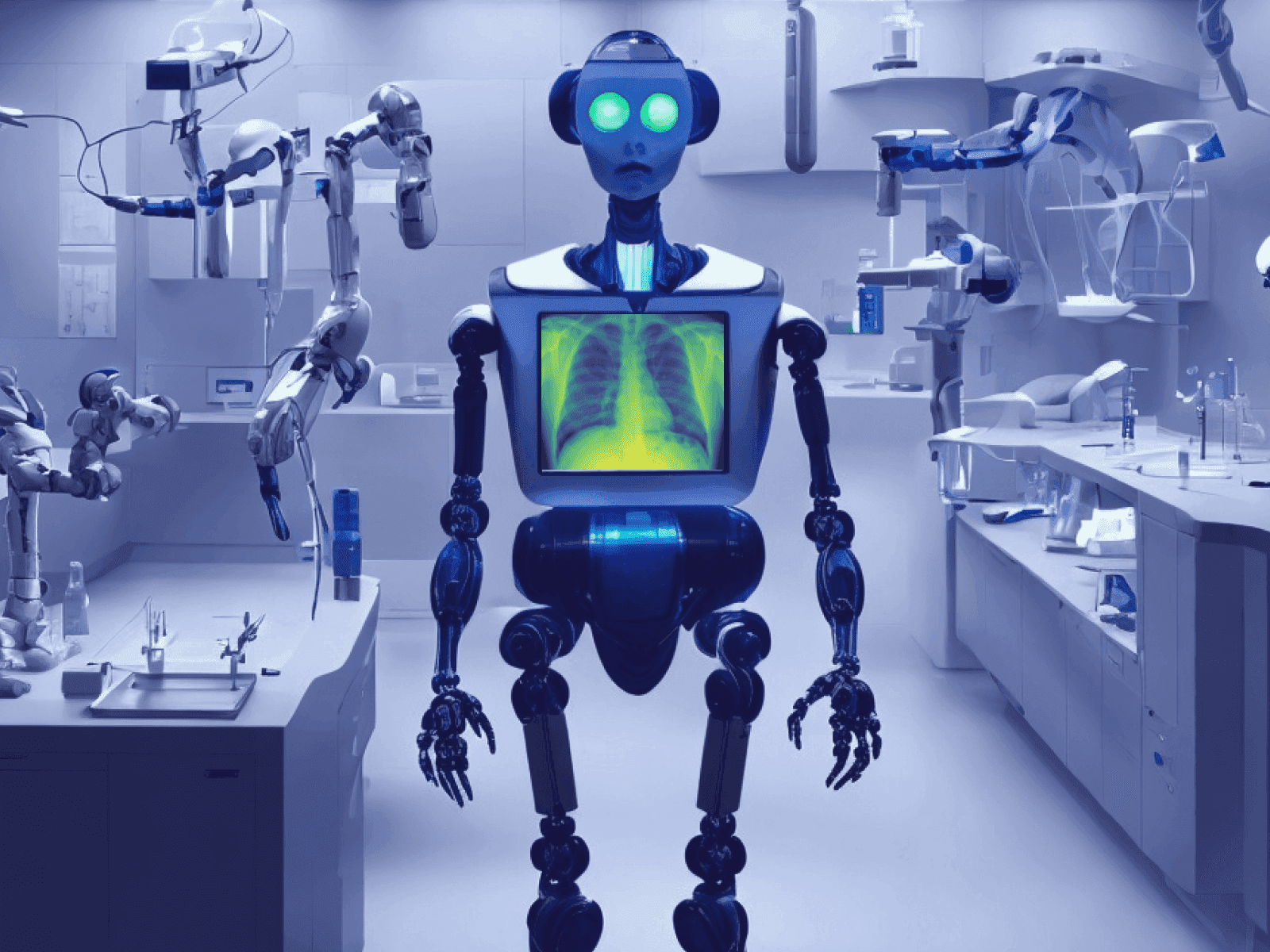
Our partners at Graphcore have run the vit-base-patch16-224-in21k ML model and trained it using 30,000 chest X-rays. Now, the model can diagnose chest diseases. In this article, we’ll tell you how to repeat Graphcore’s success with our AI infrastructure, including how to run this model on our equipment and how much it costs.

Introduction

Today’s experiment will be conducted by Mikhail Khlystun, Head of Cloud Operation, responsible for AI at Gcore. We’ll follow him step by step through running a medical machine learning (ML) model that can diagnose based on X-rays. We’ll set up the cluster, download the dataset and model, and train it. Next, we’ll test the result by checking how the model can diagnose based on test X-rays. Finally, we’ll compare the price of running the model on different flavors and find out which cluster is the most favorable to run it on.

How to run the ML model

1. Create an AI cluster to run the model. This can be done through the Gcore Control panel. Select the region, flavor, OS image, and network setting, and generate an SSH key. Click Create cluster, and we’re all set.

2. Access the cluster.

ssh ubuntu@193.57.88.205

3. Create a localdata directory for the dataset and move to it.

mkdir localdata; cd localdata

4. Create a directory in which the model is expected to find its dataset.

mkdir chest-xray-nihcc; cd chest-xray-nihcc

5. Next, we need a dataset of 112,120 chest X-rays from 30,805 patients. The dataset is available at https://nihcc.app.box.com/v/ChestXray-NIHCC. The images directory contains parts of the 42 GB archive that must be downloaded and extracted. The batch_download_zips.py script can be used to make downloading easy.

wget "https://nihcc.app.box.com/index.php?rm=box_download_shared_file&vanity_name=ChestXray-NIHCC&file_id=f_371647823217" -O batch_download_zips.py

6. Download the dataset.

python batch_download_zips.py

7. Extract the downloaded parts of the archive.

for i in $(ls -1 images_*);do tar xvf ${i}; done

8. Download the metadata file. This file contains the “correct answers”, i.e., the doctors’ diagnoses for each dataset scan. We’ll use them to train and validate the model.

Our metadata contains the following fields: image file name, detected markers, age, gender, etc. The distribution of diagnoses according to the images presented in the archive is as follows (Source: https://nihcc.app.box.com/v/ChestXray-NIHCC).

wget "https://nihcc.app.box.com/index.php?rm=box_download_shared_file&vanity_name=ChestXray-NIHCC&file_id=f_219760887468" -O Data_Entry_2017_v2020.csv

9. Check the file contents.

head Data_Entry_2017_v2020.csv

Result:

All the data is ready. Almost everything is ready to run the model.

10. Let’s move to the directory with the model code.

cd ~/graphcore/tutorials/tutorials/pytorch/vit_model_training/

11. Run the docker image with jupyter and the pytorch library that our model will work with.

gc-docker -- -it --rm -v ${PWD}:/host_shared_dir -v /home/ubuntu/localdata/:/dataset graphcore/pytorch-jupyter:3.0.0-ubuntu-20.04-20221025

After executing the command, we find ourselves inside the container. All subsequent commands have to be executed there unless clearly specified otherwise.

12. Go to the directory mounted from the host machine, where you’ll see the following contents:

For everything to work correctly, we need to replace sklearn with scikit-learn in the requirements.txt file. It can be done with any text editor or with a command:

sed -i ‘s/sklearn/scikit-learn/’ requirements.txt

13. Set an environment variable with the path to the dataset.

export DATASET_DIR=/dataset

14. Now we can run jupyter.

jupyter-notebook --no-browser --port 8890 --allow-root --NotebookApp.password='' --NotebookApp.token=''

This command starts the jupyter-notebook web server without authorization and connects only via localhost. This will require using an SSH tunnel but will eliminate unauthorized access.

15. Set up a new SSH session with our AI cluster, enabling the tunnel for port 8890. In a separate window, execute the following command:

ssh -NL 8890:localhost:8890 ubuntu@193.57.88,205

16. In the browser, follow the link

http://127.0.0.1:8890/notebooks/walkthrough.ipynb

.

We should see the following:

We’re one step away from starting the model training. Just click “Run All”.

In 15 minutes, you can see the results. Here are a few examples downloaded from the dataset:

Here are the loss function and learning_rate graphs for the training set.

The following results were obtained in the evaluation set:

Model testing

We trained the model on 112,122 chest scans. It should now have a high probability of making the correct diagnosis by processing a new image. We’ll check by adding nine new scans whose diagnoses are unknown to the model.

To do this, we’ll add more cells to the notebook with the code.

1. Let’s save the results of our model training.

trainer.save_model()
trainer.save_state()

2. Download the necessary modules.

 from transformers import AutoModelForImageClassification, AutoFeatureExtractor
from PIL import Image
import torch

3. Download feature_extractor and model from the saved files.

feature_extractor = AutoFeatureExtractor.from_pretrained(‘./results’)
model = AutoModelForImageClassification.from_pretrained(‘./results’)

4. Let’s transfer looped scans from the dataset for “diagnosing”, output it as the header for images, and add the correct value for comparison.

fig = plt.figure(figsize=(20, 15))

unique_labels = np.array(unique_labels)

convert_image_to_float = transforms.ConvertImageDtype(dtype=torch.float32)
for i, data_dict in enumerate(dataset["validation"]):
    if i == 9:
        break
    
    image = data_dict["pixel_values"]
    image = convert_image_to_float(image)
    label = data_dict["labels"]
    
    
    image_img = Image.open(data_dict["image"].filename)
    encoding = feature_extractor(image_img.convert("RGB"), return_tensors="pt")
    
    with torch.no_grad():
        outputs = model(**encoding)
        logits = outputs.logits

    predicted_class_idx = logits.argmax(-1).item()
        
    ax = plt.subplot(3, 3, i + 1)
    ax.set_title("Prediction: " + id2label[predicted_class_idx] + "|Real: " + ", ".join(unique_labels[np.argwhere(label).flatten()]))
    plt.imshow(image[0])

fig.tight_layout()

The pictures above show the model predictions and the actual diagnosis. Not all results are accurate, but the inaccuracies are within the AUCROC=0.7681 and loss=0.1875 metrics. Most of the predictions fully or partially coincide with the diagnosis made by the doctor.

Please note that, regardless of the quality of the model, an ML model is no substitute for a doctor. The model can only be a good aid in giving a preliminary result that then needs to be validated.

How much it costs

Let’s calculate how much it would cost to get involved with science and reproduce this experiment. For comparison, we’ll take the cost of running the model on three flavors:

• Minimum configuration: vPOD4 + Poplar server on a CPU60 virtual machine
• Medium configuration: vPOD4 + bare metal Poplar server.
• High configuration: vPOD16 + bare metal Poplar sever.

The names of the flavors and their cost per hour of use are given in the table.

We have divided the process of starting an ML model into two parts: preparation and training. Each measurement was repeated 10 times. The tables below show the average of the 10 attempts.

Preparation

Preparation includes downloading the dataset, extracting the images, and running the commands from the guide above. Their execution time doesn’t depend on which AI cluster you rent; it’s just a routine that you do. But the price will differ because of the flavors’ prices.

The model training includes all the actions that AI performs. Their duration depends on the flavor. The more powerful the AI cluster is, the faster it processes the data and yields results. We calculated net training and validation times using internal monitoring metrics. You can also calculate those using the %time command, which should be added as the first line to the desired cell in jupyter.

The figures show that increasing the cluster size significantly reduces the time it takes to train the model. vPOD16 was twice as fast as vPOD4.

Let’s summarize the figures to make it easy to assess the difference.

It’s worth noting that with large datasets, the time/money ratio will vary. Think of the small and large clusters like a truck and a Boeing. If cargo needs to be transported a short distance, a giant Boeing doesn’t have enough time to gain altitude and accelerate before it needs to land, so a truck can easily outrun it. But if we’re talking about really long distances (datasets), Boeing has the advantage. If your datasets are measured in hundreds and thousands of gigabytes, using vPOD16, vPOD64, and vPOD128 will show a considerable speed advantage.

If we increase our dataset 500-fold, the time to train the ML model will increase linearly. In this case, we’d get the following figures:

As you can see, the time/money ratio is very different—with a large dataset, a high configuration gives a lot of advantages. 

Conclusion

ML models are reshaping our lives. They help create pictures and game assets, write code, create text, and make medical diagnoses.

Today, we saw how you can run and train an open-source model to analyze chest X-rays in just two hours. We ran it on Gcore AI Infrastructure, which is designed to get the results of ML tasks quickly. Owing to it, training took only 6-15 minutes (depending on the selected cluster configuration), and most of the time was spent downloading the model and working with the code.

A comparison of AI clusters proved that working with a small dataset on a cluster with a minimal configuration is more profitable. When proceeding with small tasks, it’s almost as fast as a high configuration and way cheaper (we spent only $17). But the situation changes with a large dataset. If you increase the dataset 500-fold, the powerful cluster gets a huge speed advantage. It’ll handle the task twice as fast as its little brother.