Evaluating Server Connectivity with Looking Glass: A Comprehensive Guide

When you’re considering purchasing a dedicated or virtual server, it can be challenging to assess how it will function before you buy. Gcore’s free Looking Glass network tool allows you to assess connectivity, giving you a clear picture of whether a server will meet your needs before you make a financial commitment. This article will explore what the Looking Glass network tool is, explain how to use it, and delve into its key functionalities like BGP, PING, and traceroute.

What Is Looking Glass?

Looking Glass is a dedicated network tool that examines the routing and connectivity of a specific AS (autonomous system) to provide real-time insights into network performance and route paths, and show potential bottlenecks. This makes it an invaluable resource for network administrators, ISPs, and end users considering purchasing a virtual or dedicated server. With Looking Glass, you can:

• Test connections to different nodes and their response times. This enables users to initiate connection tests to various network nodes—crucial for evaluating response times, and thereby helpful in performance tuning or troubleshooting.
• Trace the packet route from the router to a web resource. This is useful for identifying potential bottlenecks or failures in the network.
• Display detailed BGP (Border Gateway Protocol) routes to any IPv4 or IPv6 destination. This feature is essential for ISPs to understand routing patterns and make informed peering decisions.
• Visualize BGP maps for any IP address. By generating a graphical representation or map of the BGP routes, Looking Glass provides an intuitive way to understand the network architecture.

How to Work with Looking Glass

Let’s take a closer look at Looking Glass’s interface.

Under Gcore’s AS number (AS199524), header, and introduction, you will see four fields to complete. Operating Looking Glass is straightforward:

1. Diagnostic method: Pick from three available diagnostic methods (commands.)
   • BGP: The BGP command in Looking Glass gives you information about all autonomous systems (AS) traversed to reach the specified IP address from the selected router. Gcore Looking Glass can present the BGP route as an SVG/PNG diagram.
   • Ping: The ping command lets you know the round trip time (RRT) and Time to Live (TTL) for the route between the IP address and the router.
   • Traceroute: The traceroute command displays all enabled router hops encountered in the path between the selected router and the destination IP address. It also marks the total time for the request fulfillment and the intermediate times for each AS router that it passed.
2. Region: Choose a location from the list of locations where our hosting is available. You can filter server nodes by region to narrow your search.
3. Router: Pick a router from the list of Gcore’s available in the specified region.
4. IP address: Enter the IP address to which you want to connect. You can type in both IPv4 and IPv6 addresses.
5. Click Run test.

After you launch the test, you will see the plain text output of the command and three additional buttons in orange, per the image below:

• Copy to clipboard: Copies command output to your clipboard.
• Open results page: Opens the output in a separate tab. You can share results via a link with third parties, as this view masks tested IP addresses. The link will remain live for three days.
• Show BGP map: Provides a graphical representation of the BGP route and shows which autonomous systems the data has to go through on the way from the Gcore’s node to the IP address. This option is only relevant for the BGP command.

In this article, we will examine each command (BGP, ping, and traceroute) using 93.184.216.34 (example.com) as a target IP address and Gcore’s router in Luxembourg (capital of the Duchy of Luxembourg), where our HQ is located. So our settings for all three commands will be the following:

• Region: Europe
• Router: Luxembourg (Luxembourg)
• IP address: 93.184.216.34. We picked example.com as a Looking Glass target server.

Now let’s dive deeper into each command: BGP, ping, and traceroute.

BGP

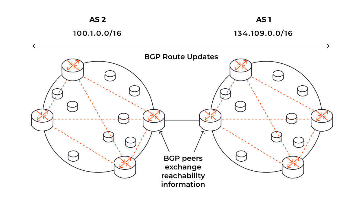
The BGPLooking Glass shows the best BGP route (or routes) to the destination point. BGP is a dynamic routing protocol that connects autonomous systems (AS)—systems of routers and IP networks with a shared online routing policy. BGP allows various sections of the internet to communicate with one another. Each section has its own set of IP addresses, like a unique ID. BGP captures and maintains these IDs in a database. When data has to be moved from one autonomous system to another over the internet, BGP consults this database to determine the most direct path.

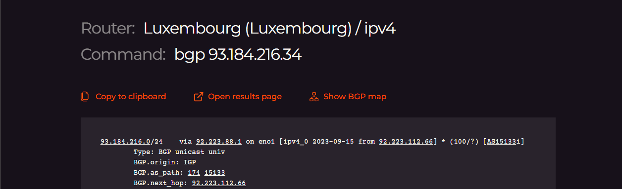
Based on this data, the best route for the packets is built; and this is what the Looking Glass BGP command can show. Here’s an example output:

The data shows two possible paths for the route to travel. The first path has numbers attached; here’s what each of them means:

1. 93.184.216.0/24: CIDR notation for the network range being routed. The “/24” specifies that the first 24 bits identify the network, leaving 8 bits for individual host addresses within that network. Thus it covers IP addresses from 93.184.216.0 to 93.184.216.255.
2. via 92.223.88.1 on eno1: The next hop’s IP address and the network interface through which the data will be sent. In this example, packets will be forwarded to 92.223.88.1 via the eno1 interface.
3. BGP.origin: IGP: Specifies the origin of the BGP route. The IGP (interior gateway protocol) value implies that this route originated within the same autonomous system (AS.)
4. BGP.as_path: 174 15133: The AS path shows which autonomous systems the data has passed through to reach this point. Here, the data traveled through AS 174 and then to AS 15133.
5. BGP.next_hop: 92.223.112.66: The next router to which packets will be forwarded.
6. BGP.med: 84040: The Multi-Exit Discriminator (MED) is a metric that influences how incoming traffic should be balanced over multiple entry points in an AS. Lower values are generally preferred; here, the MED value is 84040.
7. BGP.local_pref: 80: Local preference, which is used to choose the exit point from the local AS. A higher value is preferred when determining the best path. The local preference of 80 in the route output indicates that this route is more preferred than other routes to the same destination with a lower local preference.
8. BGP.community: These are tags or labels that can be attached to a route. Output (174,21001) consists of pairs of ASNs and custom values representing a specific routing policy or action to be taken. Routing policies can use these communities as conditions to apply specific actions. The meaning of these values depends on the internal configurations of the network and usually requires documentation from the network provider for interpretation.
9. BGP.originator_id: 10.255.78.64: This indicates the router that initially advertised the route. In this context, the route originated from the router with IP 10.255.78.64.
10. BGP.cluster_list: This is used in route reflection scenarios. It lists the identifiers of the route reflectors that have processed the route. Here, it shows that this route has passed through the reflector identified by 10.255.8.68 or 10.255.8.69 depending on the path.

Both routes are part of AS 15133 and pass through AS 174, but they have different next hops (92.223.112.66 and 92.223.112.67.) This allows for redundancy and load balancing.

BGP map

When you run the BGP command, the Show BGP map button will become active. Here’s what we will see for our IP address:

Let’s take this diagram point by point:

• AS199524 | GCORE, LU: This is the autonomous system belonging to Gcore, based in Luxembourg. The IP 92.223.88.1 is the part of this AS, functioning as a gateway or router.
• AS174 | COGENT-174, US: This is Cogent Communications’ autonomous system, based in the United States. Cogent is a major ISP.
• AS15133 | EDGECAST, US: This AS belongs to Edgecast, also based in the United States. Edgecast is generally involved in content delivery network (CDN) services.
• 93.184.216.0/24: This CIDR notation indicates a network range where example.com (93.184.216.34) is located. It might be a part of Edgecast’s CDN services or another network associated with one of the listed AS.

In summary, Gcore’s BGP Looking Glass command is an essential tool for understanding intricate network routes. By offering insights into autonomous systems, next hops, and metrics like MED and local preference, it allows for a nuanced approach to network management. Whether you’re an ISP peered with Gcore or a network administrator seeking to optimize performance, the data generated by this command offers a roadmap for strategic decision making.

Ping

The ping command is a basic, essential network troubleshooting tool that measures the round-trip time for sending a packet of data from the source to a destination and back. Ping shows the packet transfer speed and can also be used to check the node’s overall availability.

The command utilizes the ICMP protocol. It works as follows:

• The router sends a packet from the IP address to the node.
• The node sends it back.

In our case, this command shows how much time it takes to transfer a packet from the specified IP address to the node.

Let’s break down our output:

Main part:

1. Target IP: You pinged 93.184.216.34, which is the example.com IP address we are testing.
2. Packet Size: 56(84) bytes of data were sent. The packet consists of 56 bytes of data and 28 bytes of header, totaling 84 bytes.
3. Individual pings: Each line indicates a single round trip of a packet, detailing:
   • icmp_seq: Sequence number of the packet.
   • ttl: Time-to-Live, showing how many more hops the packet could make before being dropped.
   • time: Round-trip time (RTT) in milliseconds.

Statistics:

4. 5 packets transmitted, 5 received: All packets were successfully transmitted and received, indicating no packet loss
5. 0% packet loss: No packets were lost during the transmission
6. time 4005ms: Total time taken for these five pings
7. rtt min/avg/max/mdev: Round-trip times in milliseconds:
   • min: minimum time
   • avg: average time
   • max: maximum time
   • mdev: mean deviation time

To summarize, the average round-trip time here is 87.138 ms, and the TTL is 52. RTT of less than 100 ms is generally considered acceptable for interactive applications, and TTL of 50 is considered a good value. No packet loss suggests a stable connection to the IP address 93.184.216.34.

The ping function provides basic, vital metrics for assessing network health. By offering details on round-trip times, packet loss, and TTL, this command allows for a quick yet comprehensive evaluation of network connectivity. For any network stakeholder—whether ISP or end user—understanding these metrics is crucial for effective network management and troubleshooting.

Traceroute

The Looking Glass traceroutecommand is a diagnostic tool that maps out the path packets take from the source to the destination, enabling you to identify potential bottlenecks or network failures. Traceroute relies on the TTL (Time-to-Live) parameter, which basically determines how long this packet can stay in the network. Every router along the packet’s path decrements the TTL by 1 and forwards the packet to the next router in the path. The process works as follows:

1. The traceroute sends a packet to the destination host with TTL value of 1.
2. The first router that receives the packet decrements the TTL value by 1 and forwards the packet.
3. When the TTL reaches zero, the router drops the packet and sends an ICMP Time Exceeded message back to the source host.
4. The traceroute records the IP address of the router that sent back the ICMP Time Exceeded message.
5. The traceroute then sends another packet to the destination host with a TTL value of 2.
6. Steps 2-4 are repeated until the traceroute routine reaches the destination host or until it exceeds the maximum number of hops.

Now let’s apply this command to the address we used earlier. The traceroute command will test our target IP address with 60-byte packets and a maximum of fifteen hops. Here’s what we get as output:

Apart from the header, each output line consists of the following information, labeled on the image below:

1. IP and hostname: e.g., vrrp.gcore.lu (92.223.88.2)
2. AS information: Provided in square brackets, e.g., [AS199524/AS202422]
3. Latency: Time in milliseconds for the packet to reach the hop and return, e.g., 0.202 ms

In our example, traceroute traverses through three different autonomous systems (AS):

1. AS199524 (GCORE, LU): The first two hops are within this AS, representing the initial part of the route.
2. Hops 3 and 4 fall under the private IPv4 address space (10.255.X.X), meaning the hops are within a private network. This could be an internal router or other networking device not directly accessible over the public Internet. Private addresses like this are often used for internal routing within an organization or service provider’s network.
3. AS174 (COGENT, US): Hops 5 to 9 are within Cogent’s network.
4. AS15133 (EDGECAST, US): The final hops are within EdgeCast’s network, where the destination IP resides.

To sum up, the traceroute command offers a comprehensive view of the packet journey across multiple autonomous systems. Providing latency data and AS information at each hop, it aids in identifying potential bottlenecks or issues in the network. This insight is invaluable for anyone looking to understand or troubleshoot a network path.

Conclusion

Looking Glass is a tool for pre-purchase network testing, covering node connectivity, response times, packet paths, and BGP routes. Its user-friendly interface requires just a few inputs—location, target IP address, and the command of your choice—to deliver immediate results.

Based on your specific needs, such as connectivity speeds and location, and the insights gained from Looking Glass test results, you can choose between Gcore Virtual Dedicated Servers or Dedicated server hosting, both boasting outstanding connectivity.